"Geographic Expansion-Staff Hiring" Problem in Excel (With Solution)

Published on Jul 27, 2019 ⸱ 6 min read ⸱ 20 views

Please ignore the lame attempt at naming a rather mundane problem. I tried, in wane, to name it something cool like the "Traveling Salesman Problem".

Recently, while working on a financial model for a startup, I came across a rather peculiar modelling problem I had never encountered before. This problem really stretched my capabilities and command over Excel (FWIW). It took me almost 2 days to figure a solution, which came to me when I was not thinking of the problem. Irony.

The problem statement of the model is as follows: For a B2B SaaS startup (let's call it Startup X) it's customer acquisition is largely driven by offline feet-on-street. It intends to acquire customers city by city, entering a new city once it has built a foundation in each city. The feet-on-street staff hiring is done in a particular manner without following any specific pattern.

Now, the problem is how do we build a programmatic model in excel for a three (for example) city expansion where we can simulate the staff requirement/roll out based on a dynamic launch date in each new city.

Take a moment and think about the problem. If you fully understand the problem, I invite you to take a shot at solving the problem. Here's a dummy excel sheet you can download to work on. I've included the solution below, in case you give up.

Breaking down the problem and the solution as below:

Problem:

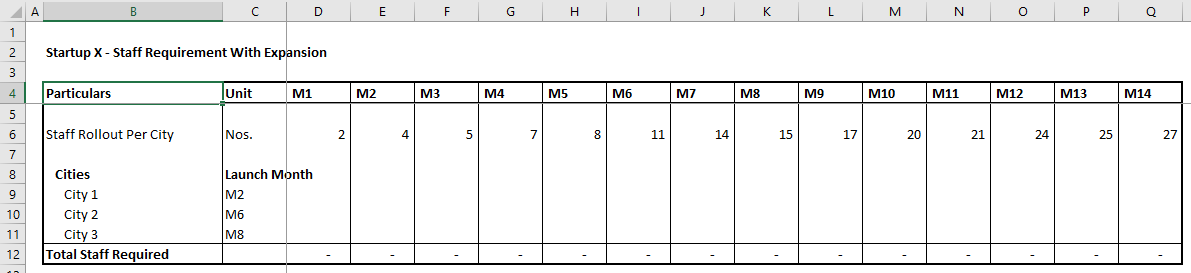
The model (snapshot above) has a certain period of months (M1 to M14 in this case) over which Startup X will expand in three cities i.e. City 1, City 2 and City 3. In each city, Startup X will hire staff in the same manner as listed in Row 6 i.e. Staff Rollout per city. The "Launch Month" (Cell: C9 to C11) is a drop down to select from months M1 to M14.

Example: Consider an example where Startup X will commence operations in city "City 1" in month "M2". It will begin hiring as per the requirement stated in "Row 6", starting from cell E9 onward. Therefore, the staff requirement for "City 1" will be cell E9=2, F9=4,G9=5.... and so on. Similarly for Cities 2 & 3 as per the launch months of "M6" and "M8" and staff roll out in City 2 will begin from M6 onward and City 3 from M8 onward.

The easiest solution for this is to hard code the solution based on the launch month of that city. i.e. inputting the formula Cell E9=D6, F9=E6, G9=F6... and so on till M14. Easier still, is copy pasting row 6 to row "City 1" starting from "M2". But that's inelegant and any self respecting Financial Modeller (if that's a word) will scoff at the thought of that.

Now for the sake of evaluation, I want to see the total staff requirement if I advance "City 2"'s launch month by 2 months. i.e. I change "City 2" launch month from "M6" to "M4". Since we have hard coded the formulae to display values starting from "M6", "M4" and "M5" for "City 2" will show zero staff and "M6" onward will continue to show the same values. You need to do a lot of manual work to change the employee roll out.

That's, again, not the desired outcome. The staff requirement should dynamically change if I change the launch month of any city to any month from the model. That's the point of a model after all - being able to simulate different scenarios.

Take a moment again and think about a solution. Try various formulae to achieve our goal. Use the template. I've tried dozens and failed many times except one. Now, unlike Dr. Strange, I'm not saying there's only one solution.

If you're unable to think of a solution, scroll on.

My Solution:

Let's breakdown the problem we're trying to address:

If the launch month is equal to the current month, we start with the staff requirement in the current cell. If the launch month is not the current month, then we do not need any staff.
If the first condition is satisfied, then we need to insert the staff requirement of the following months in the cell after the current month. Again, if the condition is not satisfied, then we do not need any staff.

Breaking down the problem statement this way gives some clues i.e. we need to use nested condition formula. The formulae are simpler than I thought they would be.

Addressing the first condition as above, for the first month "M1" in "City 1" we could use the simple =IF() formula as below:

=IF($C9=D$4,$D$6,0)

Here, we are simply saying, if the Launch Month is equal to the current month, then input the first Staff Requirement.

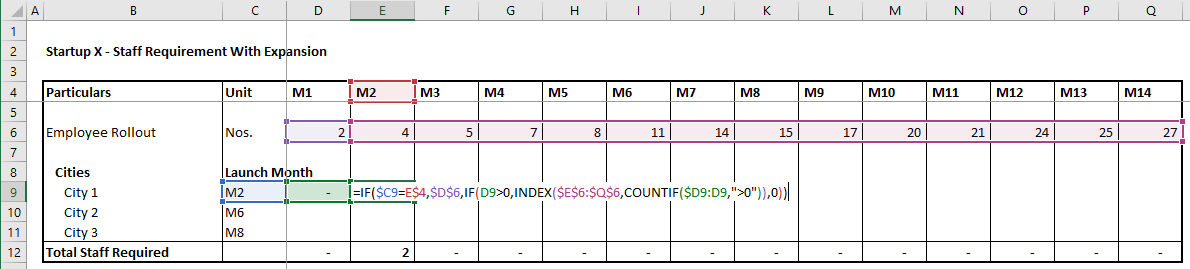
The Second part is where it gets tricky. To address the second clause, we need to input the following formula in the adjacent cell:

=IF($C9=E$4,$D$6,IF(D9>0,INDEX($E$6:$Q$6,COUNTIF($D9:D9,">0")),0))

Yes, I know! The formula looks dangerous. Trust me, it's just the opposite.

In this adjacent cell, we input the the above formula. But if you notice the formula, we've used the first IF() function and instead of the "value if false" result, we input another nested IF() formula: IF(D9>0,INDEX($E$6:$Q$6,COUNTIF($D9:D9,">0")),0)

This formula is telling the cell that If the previous cell is greater than 0, then from the range of our "Employee Hiring" i.e. Row 6, begin inserting the employee count and offset the INDEX of the COLUMN by the number of cells greater than 0. It's quite simple really.

If you're not familiar with INDEX() function, read this explainer from Microsoft Support.

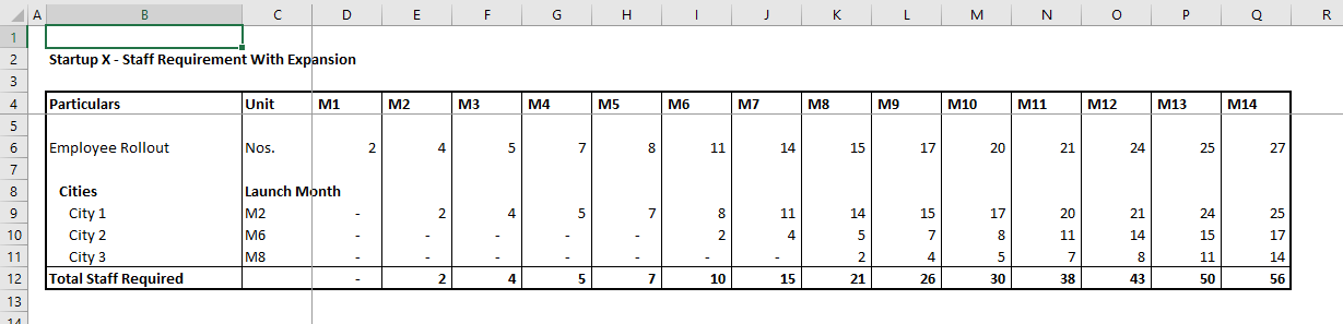
You can download the excel file with the solution here. In the excel file, you can change the launch month from the drop down and see the employee roll out changes automatically. Below is a screenshot of the solution.

If you think of another solution, please share it. Would like to learn the other ways of solving this (irritating) problem.

Look forward to hearing your comments on this.

Onward.

Note: All blogs posts till 2022 were migrated to this platform (react+next+tailwind). While all efforts were made to migrate wihtout any loss, the migration lost some images and broke a bunch of links in old posts. If you spot anything amiss, please notify me?